
Recently, a friend of mine had a problem. He wanted to model the response of an isotropic, linear elastic medium to a point defect. It sounds simple enough. (The following physics isn’t really relevant to this blog post, by the way.) First, we write down the strain tensor \(u_{ij}\) in terms of the displacement field \(u_i\), or
\[u_{ij}=\frac12(\partial_iu_j+\partial_ju_i+\partial_iu_k\partial_ju_k)\]
Then, the total free energy of the medium can be compactly expressed by
\[F=\frac12\lambda u_{ii}u_{jj}+\mu u_{ij} u_{ij}\]
In order to find the response of the elastic medium, we can use the Euler–Lagrange equations to minimize the free energy with respect to the displacement. Since \(F\) only depends on derivatives of \(u_i\), the three differential equations that, solving, would give the response of the system to a point defect are
\[\partial_j\frac{\partial F}{\partial\partial_ju_i}=\delta(x)\]
Great! So what’s the problem? Well, we’ve yet to write down these equations explicitly, and the simple form above belies a tangled mess. Even after running Mathematica’s Simplify routine on the system, the result is not pretty. “So?”, you say “Just let the computer take care of it!” Again, a subtlety remains: this system, difficult to solve numerically as is, would be vastly simplified if we could enforce the spherical symmetry of a point defect. Then the displacement would simply take the form \(\mathbf u=u(r)\;\hat{\mathbf r}\), and we would have on ODE, rather than three coupled PDEs. To do this, we need to write the equations above in spherical coordinates.
Unfortunately, there is no easy way to transition differential equations in one coordinate system, like those above, into differential equations in a second coordinate system. Sure, with Mathematica’s CoordinateTransformData we can rewrite the coordinates themselves easily enough, but what about the derivative operations? One look at the Wikipedia page for translating \(\nabla\) between systems shows that this task is nontrivial for just one measly partial derivative operator, but in an equation like ours there are mixed derivatives of every type! A systematic way would be very valuable.
And so that’s what I set about to do. First, and most basically, we need a way of expressing derivatives with respect to our old coordinates, e.g., \(\partial_x\), in terms of our new coordinates, e.g., \(r,\theta,\phi\). The chain rule comes to the rescue, supplying us with the general formula:
\[
\frac\partial{\partial x_i}=\frac{\partial y_j}{\partial x_i}\frac\partial{\partial y_j}
\]
How do we retrieve the functions \(y_j(x)\) in a systematic way? Fortunately, Mathematica has us covered for that one: the built-in CoordinateTransformData will return the mappings, in the conventional order, from any two coordinates systems in Mathematica’s database, which is pretty exhaustive. For instance, if we wanted the spherical coordinates \(r, \theta, \phi\) from ordinary Cartesian coordinates, we would run
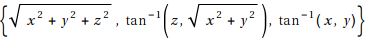
which is exactly what we expect. The final argument, here {x, y, z}, just tells Mathematica the labels it should use for the old coordinates. What we’d like is a function which takes these coordinate mappings, differentiates them, and adds them up with the associated differential operators, as per the chain rule. The following function, dC, does just that:
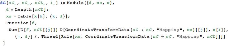
This function takes as input the old coordinates oC, the new coordinates nC, the list of labels for the new coordinates nCL, and the index i of the old coordinate to differentiate. It returns a function that is completely analogous to Mathematica’s D function, but with only one argument. For instance,


would return the derivative of f with respect to x[1] as a function of the spherical coordinates \(r, \theta, \phi\).
Now that we have a rudimentary way of translating derivatives, we still need a way to get those derivatives into Mathematica expressions. Of course, we’d like to use our favorite Wolfram tool: pattern matching! In order to do this, we need to understand something about the way that derivatives actually appear in expressions. The D[f, x] notation only exists on the command line: in an evaluated expression, the function of relevance is Derivative, which looks like
Derivative[n1, n2, n3, ..., nm][f][x1, x2, x3, ..., xm]This expression takes a function of \(m\) variables, \(f(x_1,x_2,\ldots,x_m)\), and differentiates it \(n_i\) times with respect to \(x_i\). In this compact notation, all mixed partial derivatives can be expressed easily, without nesting functions! Of particular convenience, it allows us to find and replace only the head of the derivative expression without having to do silly matching inside it.
Which leads us to our coordinate-changing operator, derivativeC. This operator is going to need additional arguments so that it knows what it’s transforming from and to, and should, after those arguments, take the same arguments as the Derivative function. Then, for every partial derivative of a certain type, it should nest the function argument inside ni of the single derivative transforms dC for that coordinate. And that is precisely what follows, albeit in a condensed form:
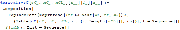
This does the job. For instance,


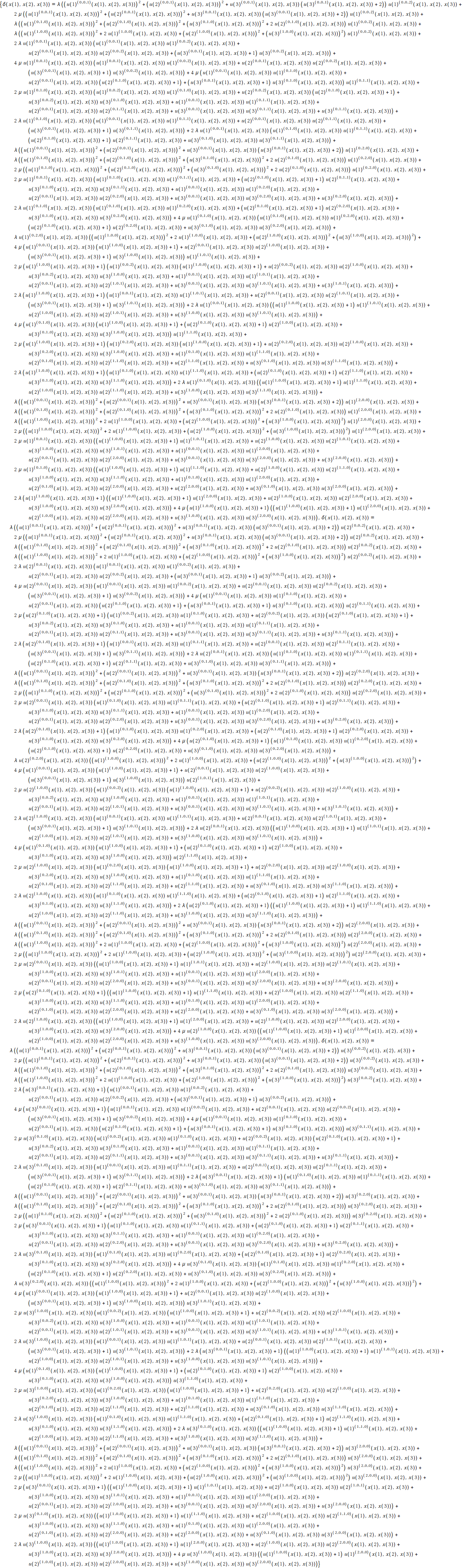
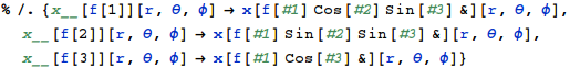
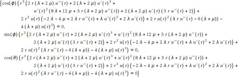
We can also run this routine on our large set of differential equations from above, translating them to differential equations in spherical coordinates. Of course, this by itself is not a simplification; if anything, the expression is far more complicated. (I tried to upload an image of the unsimplified equations, but got this.) But now we can easily enforce our constraint! Because our function is nested in Derivative expressions, we need to replace it in a somewhat convoluted way:
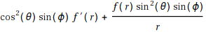
Making this transformation to our elastic differential equations above, we find them greatly simplified, and reduced to only one equation! One numeric solution is shown at the head of this post. Of course, no one reading this cares about vacancies (probably), and so the useful Mathematica code is also online, here. Enjoy!