Recently, while tutoring the Electromagnetism & Optics class at HMC, another tutor presented me with an unexpected problem they couldn’t seem to resolve: simply deriving the electrostatic potential of a point charge. I will describe their method, which took me a rather long time to find the fault in.
Let the origin of our coordinate system lie at the charge. Using Gauss’ law, it is easy to show that the electric field is given by
\[\mathbf E(\mathbf r)=\frac1{4\pi\epsilon_0}\frac q{r^2}\,\hat{\mathbf r}\]
The electric potential relative to infinity is then, by definition,
\begin{equation}
\varphi(\mathbf r)=-\int_{\mathbf a}^{\mathbf r}\mathbf E(\mathbf s)\cdot\mathrm d\mathbf s\label{potential}
\end{equation}
where it is understood that \(\mathbf a\) is located ‘at infinity.’ Since
the electric field is conservative, this integration may be taken over any path
between \(\mathbf a\) and \(\mathbf r\). We choose the natural path, that
is, the one moving radially inwards towards \(\mathbf r\). In that case, \(\hat{\mathbf r}\cdot\mathrm d\mathbf s=(-1)\;\mathrm ds\), since the direction of the path is radially inwards, and the limits of integration are from \(\infty\) to \(r\), yielding
\begin{align*}
\varphi(\mathbf r)
&=-\int_\infty^rE(s)(-1)\,\mathrm ds
=\frac1{4\pi\epsilon_0}\int_\infty^r\frac q{s^2}\,\mathrm ds\\
&=\frac1{4\pi\epsilon_0}\left[-\frac qs\right]_{s=\infty}^{s=r}
=-\frac1{4\pi\epsilon_0}\frac qr
\end{align*}
The astute reader will notice that this is the negation of the correct answer. What happened?
The answer lies in the specific application of vector calculus. Really, what is \(\mathrm d\mathbf s\)? To formally evaluate \eqref{potential}, we need to parameterize a path \(\mathbf s(t)\). Then, the integration would become \[ \varphi(\mathbf r)=-\int_{\mathbf s^{-1}(\mathbf a)}^{\mathbf s^{-1}(\mathbf r)}\mathbf E(\mathbf s)\cdot\frac{\mathrm d\mathbf s}{\mathrm dt}\,\mathrm dt \] An obvious parameterization is given by \[ \mathbf s(t)=(t,0,0) \] In this case, the limits of integration are the same as before. Most notably, it is now clear that \(\mathrm d\mathbf s/\mathrm d t=\hat{\mathbf x}\), so that, since this path is along the \(x\)-axis, \(\hat{\mathbf r}\cdot(\mathrm d\mathbf s/\mathrm dt)=1\). The earlier integration then becomes \[ \varphi(\mathbf r) =-\int_\infty^rE(t)\,\mathrm dt =\frac1{4\pi\epsilon_0}\frac qr \] which is the correct answer.
The failing of the first response is due to a nontrivial and unintuitive property of the object \(\mathrm d\mathbf s\). This vector does not point in the heuristic direction of integration, something which is made clear when the path is parameterized formally. The mistake is obvious in hindsight. But where does this incorrect understanding of vector calculus come from in the first place?
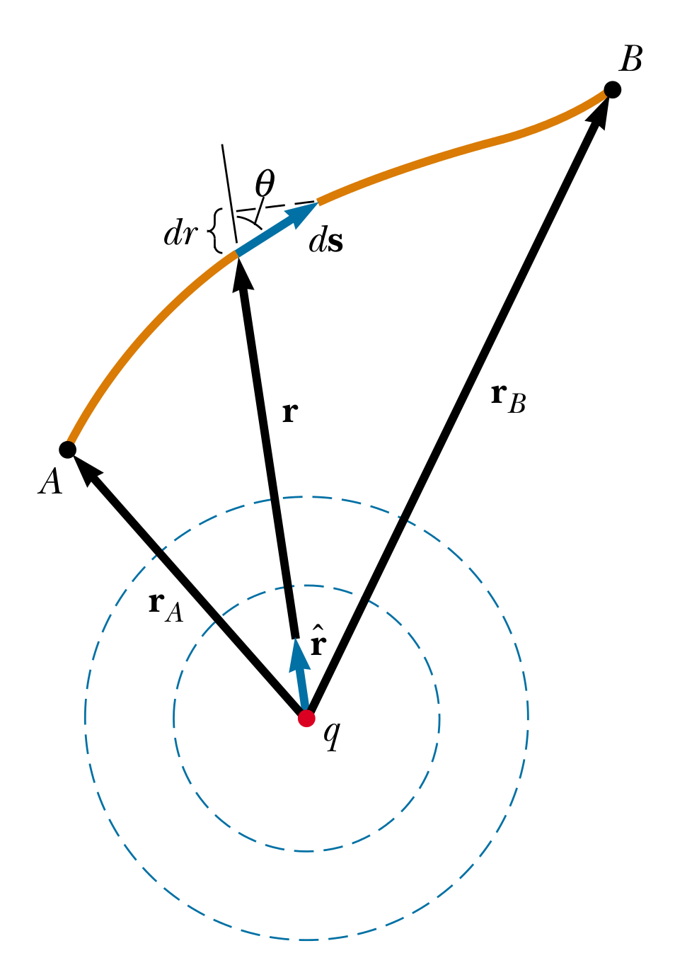
Below is the figure from the latest edition of Halliday, Resnick, and Krane’s popular introductory text on E&M. It details graphically the integration of an electric field from \(A\) to \(B\) along the orange path. Here, \(\mathrm d\mathbf s\) is featured pointing along the path in the direction from \(A\) to \(B\). This fact is taken for granted in the accompanying text, as is usual of the more rigorous mathematical substance. However, in this case, the usual intuitive mathematics is insufficient for even a working understanding. Unfortunately, HRK does not offer an alternative.
This type of intuitive treatment of mathematics that lacks rigor is common throughout physics, and is by no means a bad thing. In many cases, the requisite understanding comes easily from such a treatment and valuable time is saved by not carrying out arduous proofs or constructions. My point is that when producing such a treatment, one must be careful. An incomplete mathematical picture can lead to an incomplete or even inconsistent physical one.